You say Potato, I say 110

I was re-reading the Rectified LpJEPA paper early this week and it got me thinking - this paper allows us to regularize model outputs to match a desired global distribution. What other embedding spaces might we care about?

The first thing to come to mind was the concept of semantic hashing. This is in many ways the pre-cursor to RAG systems, and focuses on the generation of a series of bits associated with the semantic meaning of some input data, where an efficient bit-counting metric can be used (e.g. Hamming distance) to identify documents similar to a query. This use of a binary representation and an efficient metric should allow incredibly fast retrieval when combined with algorithms such as PyNNDescent (or HNSW, I just love PyNNDescent’s explainer page).

This blog post is the first in a (hopefully) 2-parter which explores using the same technique as Rectified LpJEPA to regularize a model into creating a binary embedding space.

A primer on Rectified LpJEPA Link to heading

For those who aren’t as obsessed as I am with representation learning, Rectified LpJEPA is a follow-up paper by Yilun Kuang out of New York University, co-authored by Yash Dagade, Tim G. J. Rudner, Randall Balestriero, and Yann LeCun.

Balestriero and LeCun recently(ish) authored another exciting paper, LeJEPA, which proposed that we should train representation learning systems such that the resulting embeddings conform to a pre-defined distribution. They then identified the Isotropic Gaussian as the ideal distribution for embedding spaces to maximise the power of linear probing (whether this means ideal in general is a slightly different question, but it’s very logical!). They achieve this using a new distribution matching regularization to the representation learning loss function, SIGReg, implemented using the Epps-Pulley test statistic.

The follow-up, Rectified LpJEPA, posits that inducing sparsity into this distribution will improve representation efficiency. I’m not necessarily sold on that aspect from their arguments yet (but keen to be wrong!); instead, for me, their key contribution is the introduction of RDMReg. This is an extension to SIGReg which creates a regularization term guiding our embedding space to match any desired distribution. This effectively works by sampling from the target distribution for each batch and then, via “the Cramér–Wold device” (which states that if two distributions look identical under every 1-D projection, they’re the same distribution), enforcing that the batch embeddings look as similar as possible to this random sample, over multiple linear projections.

Sorry if I lost you there - the take-home is that this regulariser says something along the lines of “what I have should look like what I want, no matter how you slice it”.

Why this (might) allow us to do semantic hashing Link to heading

We have a desired distribution of points in embedding space (vertices on a hyper-cube, if that’s how you think), and we have a way to nudge our model to place points to mimic that distribution (RDMReg). If the regularization works, we should then be able to quantize our output embeddings into a simple byte array for storage and retrieval without significant quality degradation - we can use this regularization to maximise the Shannon entropy of our embedding space while leveraging a distance-based loss to move semantically similar input (e.g. from augmentations that do not change the “meaning” of an item) data closer together.

The code to generate samples from our desired embedding distribution is straightforward:

def generate_binary_targets(shape, device, sparsity: float=0.5):
    """Generate examples of a binary distribution with points
    at vertices on the {-1, 1} hyper-cube.
	
    Parameters
    ----------
    shape: tuple[int, ...]
        The desired output shape
    device: str
        Torch device ('cpu', 'cuda', etc.)
    sparsity: float, default=0.5
        The desired weighting of zeros to ones.
    """
    return (torch.rand(shape, device=device) > sparsity).int() * 2 - 1

And the remaining code is all about implementing RDMReg - which needs a function to determine slices to take, for example slicing from a uniform hyper-sphere:

def sample_uniform_sphere(
    n_samples: int,
    d: int,
    device='cpu',
    dtype=torch.float32,
) -> torch.Tensor:
    """
    Sample random projection vectors from the uniform distribution
    on the hypersphere with dimension ``d``.

    Parameters
    ----------
    n_samples: int
        Number of vectors to sample
    d: int
	      Dimension of each vector
    device: str
    		Torch device ('cpu', 'cuda', etc.)
    dtype: torch.dtype
    		Data type (default: torch.float32)

    Returns
    -------
    vectors
        Tensor of shape (n_samples, d) with each row on the unit ℓ2 sphere
    """
    # z ~ N(0, I_d)
    z = torch.randn(n_samples, d, device=device, dtype=dtype)
    # ||z||_2 per sample
    norms = z.norm(p=2, dim=1, keepdim=True)
    # normalize onto surface of hypersphere
    c = z / norms
    return c

And the regularizing loss function itself

def distribution_matching_regularizer(
    embed: torch.Tensor,
    distribution_targets: torch.Tensor,
    n_projections: int = 128,
    sample_projections: Callable[
        [int, int, str | torch.device, torch.dtype], torch.Tensor
    ] = sample_uniform_sphere,
) -> torch.Tensor:
    """Compute a distribution-matching loss, RDMReg, to move the
    items in ``embed`` closer to the distribution used to sample
    ``distribution_targets``.
    
    Parameters
    ----------
    embed: torch.Tensor
        The embeddings to regularize
    distribution_targets: torch.Tensor
        A sample of points drawn from the target distribution. These
        should be regenerated for each time this function is called.
    n_projections: int
        The number of linear slices to take
    sample_projections:
        How slices should be sampled
    
    Returns
    -------
    torch.float32
        The loss value.
    """
    batch_size, n_dims = embed.shape
    # Sample N projections
    c = sample_projections(
        n_projections,
        d=n_dims,
        device=embed.device,
        dtype=embed.dtype,
    )

    # Project generated targets
    target_projections = distribution_targets @ c.T

    # Sort target projections
    target_projections, _ = torch.sort(target_projections, dim=0)

    # Project embeddings
    embed_projections = embed @ c.T

    # Sort projected embeddings
    embed_projections, _ = torch.sort(embed_projections, axis=0)

    # L2-norm distance from target to embed projections
    return (
        torch.pow(target_projections - embed_projections, 2).sum()
        / batch_size
    )

We can then define a standard loss function, such as moving all instances of a label towards the group centre, or minimising pairwise distances. The important thing here is that without distribution_matching_regularizer we would have been vulnerable to mode collapse, as without an outwards pressure (as is achieved using a triplet loss on a local scale, and distribution matching losses on a global scale) we are not engineering a useful embedding space.

A Quick Smoke Test Link to heading

This sounds very clever and a bit magic, which should immediately make you suspicious. I found it quite hard to visualise how RDMReg would be nudging embeddings. We can run a very simple smoke test of the method to check that the regulariser is indeed producing the desired effect by creating a simple MLP which performs a dimensionality reduction, where the loss function is purely the regularizer.

I set up a quick experiment to project samples drawn from an N-dimensional Gaussian to an E-dimensional binary space, with a small MLP. By tracking the mean absolute distance from any output embedding to the nearest unit hyper-cube vertex we can ensure that, as training progresses, our model learns to map to the desired space.

Watching this happen the first time felt magical - binning the embedding values in a batch produces plots a bit like this (I log this histogram in the terminal but can’t copy it nicely here), where we can see the regulariser in action (epochs have been altered for illustrative purposes):

Epoch 0:  ▁▁▁▁▁▃▇▁▁▁▁▁
Epoch 1:  ▁▁▁▁▁▆▇▁▁▁▁▁
Epoch 3:  ▁▁▁▃▅▆▇▅▃▁▁▁
Epoch 4:  ▁▂▃▅▆▇▆▆▅▃▂▁
Epoch 5:  ▁▂▄▇▆▆▆▆▆▄▂▁
Epoch 6:  ▁▁▃▇▄▄▄▅▅▄▁▁
Epoch 7:  ▁▁▂▇▃▂▃▃▅▃▁▁
Epoch 8:  ▁▁▁▇▂▂▂▂▅▂▁▁
Epoch 9:  ▁▁▁▇▁▁▁▁▆▁▁▁

We can alternately visualize this as the mean L1 distance from each embedded item in a batch to its nearest vertex:

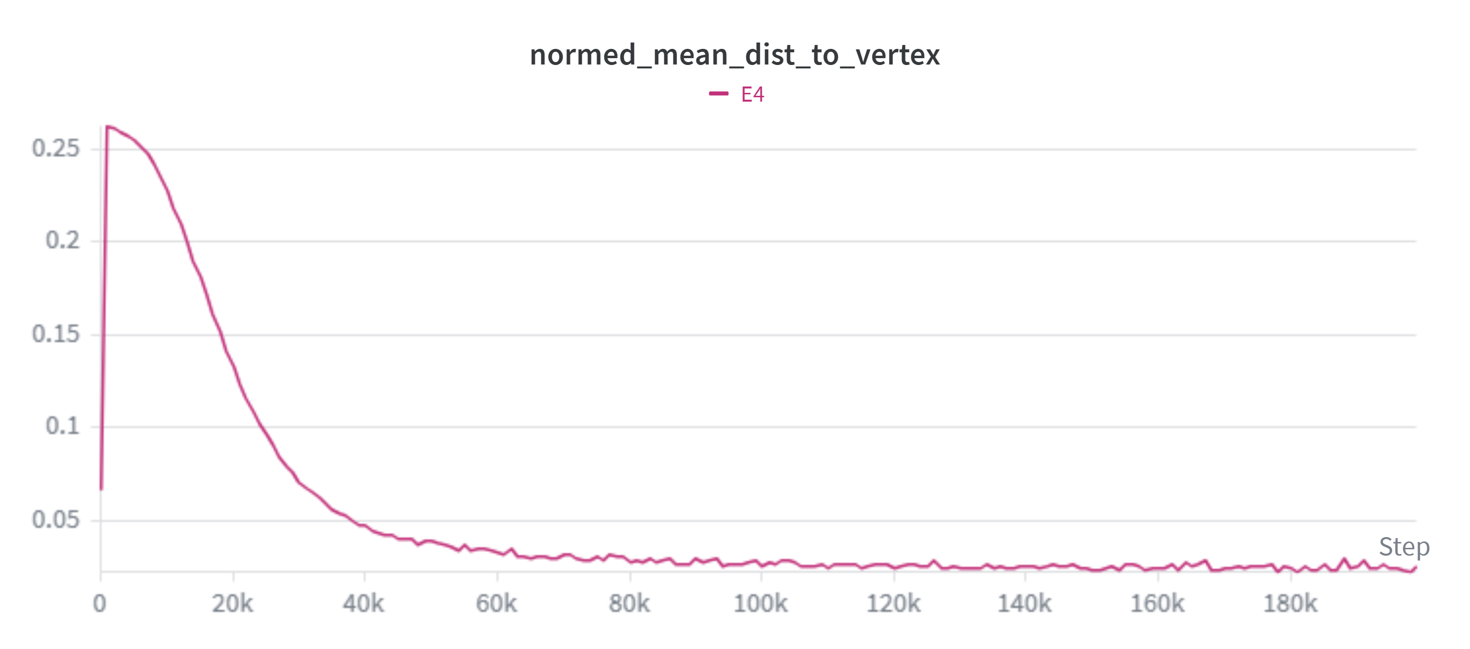
Unfortunately, while this setup works well for low output dimensionality, convergence takes increasingly longer as our embedding dimensionality (E) increases:

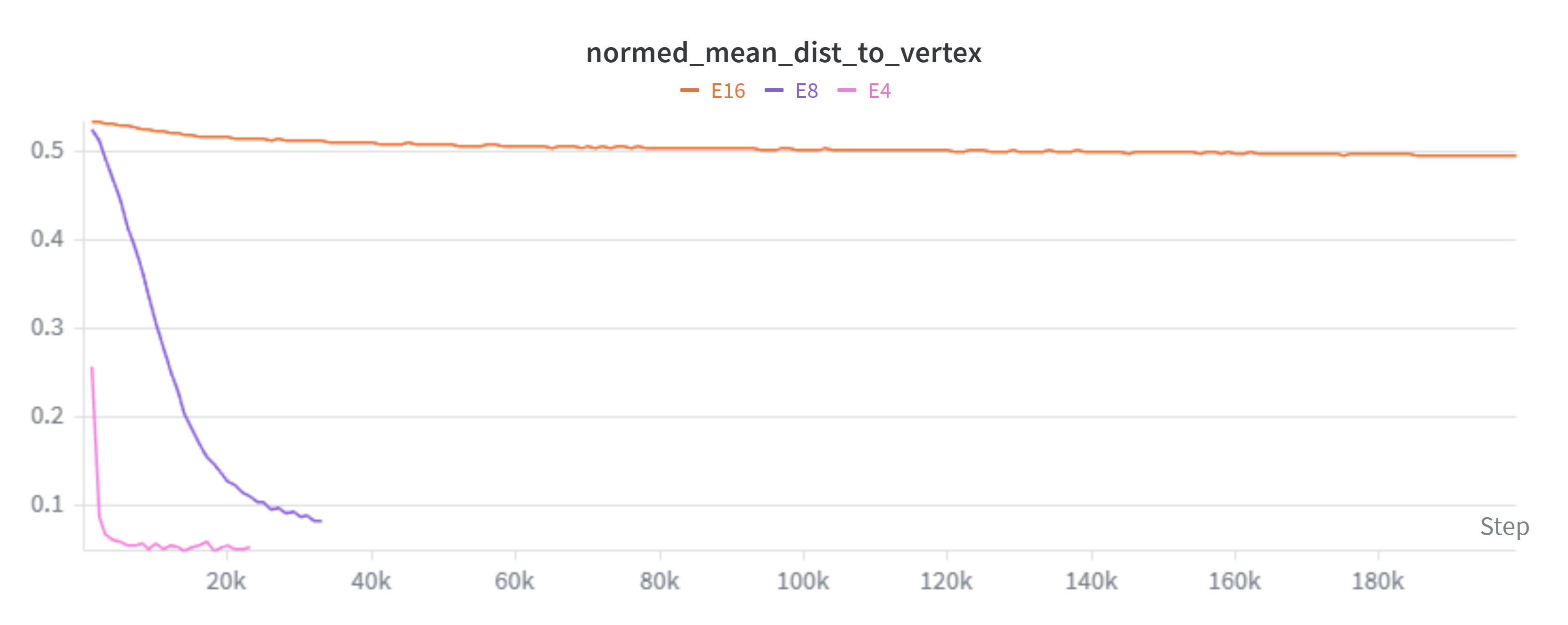
Not ideal given we’d like to get up to thousands of dimensions!

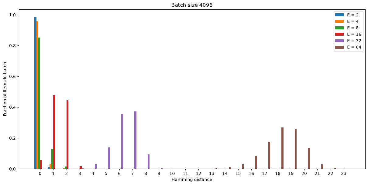
Let’s dig into this problem: this run has a batch size of 4096 items, the total number of possible hashes for E=16 is 2^16 = 65_536. In each batch it’s incredibly unlikely that the true “vertex” we should be mapping each item to will be present (as shown below), and so the item will end up trying to minimise its distance to many vertices. Since our targets are always extrema (unlike a smooth distribution), we end up with points at a muddy average rather than a clean {-1, 1}!

To demonstrate that as dimensionality increases we end up with worse targets for RDMReg, let’s assume that for each element in a batch there is some “perfect hash” that it should try to gravitate to - the distribution of these hashes will be identical to our target distribution. If we therefore take two samples from our target distribution (one for this perfect hash and another for the RDMReg targets), and match each item up from the first sample with the nearest item from the second, such that we minimise the sum of total hamming distances across matches (the well-studied linear sum assignment problem), we can see how the distribution of distances between pairs changes as our dimensionality changes for a fixed batch size:

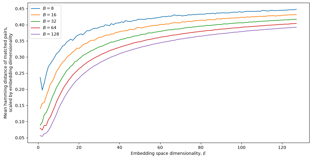
The graph shows that our random projections will only ever be consistently pulling in the correct direction for our target hash at very low dimensions, with increasing dimensions having higher and higher distances. In fact even the ratio of mean distance to dimensionality gets worse as dimensionality increases, as shown here for different batch sizes (target samples have increasingly more incorrect bits):

Instead of using our full dimensionality $E$, what if we ensure that only a handful of dimensions are “active” for any projection ($E_\text{active} \ll E$)? We can choose this number of active dimensions such that we’d expect that our sample of N targets will contain a good match for almost all of the items in a batch. For instance, as shown in the bar chart above, a batch size of 4096 might mean we have to limit ourselves to $E_\text{active}=8$ at most, to ensure ~80% of items will be moved towards the correct point for all projections.

But we must be cautious, here be dragons! By restricting to a subset of random projections we’re no longer able to benefit from the Cramér–Wold theorem underpinning RDMReg. To illustrate this, consider two random vectors, x and y, both with 3 dimensions and entries of {-1, 1}, where x is totally random

import random

BITS = [-1, 1]
def x():
    return (
        random.choice(BITS),
        random.choice(BITS),
        random.choice(BITS),
    )

but y has a 3rd dimension which is the product of its 1st and 2nd (i.e. y[0] and y[1] are conditionally negatively dependent given y[2]):

def y():
    y0 = random.choice(BITS)
    y1 = random.choice(BITS)
    y2 = y0 * y1
    return (y0, y1, y2)

A trivial comparison arises if we use a projection vector of [1, 1, 1]: the discrepancy becomes immediately apparent, since x can have value (-1, -1, -1) with probability 1/8, but y would have probability 0.

However, constraining to projection vectors where any one of the three axis is zero (e.g. [1, 1, 0], [1, 0, 1], …), we cannot differentiate between these two distributions. There is no available slice which will produce different distributions between x and y.

This opens us up to a very annoying form of mode collapse where the model will prefer to learn dimensions that are conditionally dependent, which we will need to address before we can move forward.

What we need is a mechanism that prevents any two items from collapsing to the same hash unless we explicitly want them to. A loss that operates on a small scale, creating an inflationary pressure preventing mode collapse, without imposing on the overall structure of the embedding space.

I’m still grappling with the design of this local loss: I’ve tried various metrics (from a naïve Euclidean pressure to a custom scaled cosine distance to various forms of triplet loss to a bit of Claude-generated madness involving a lot of $\tanh^{-1}$). I’m excited to explore more and see if this is a nut that can be cracked!